Slope stability analysis: The term slope means a portion of the natural slope whose original profile has been modified by artificial interventions relevant with respect to stability. The term landslide refers to a situation of instability affecting natural slopes and involving large volumes of soil.
Introduction to stability analysis
The resolution of a stability problem requires taking into account field equations and constitutive laws. The first ones are equilibrium equations, the second ones describe the behavior of the soil. These equations are particularly complex since the soil is made of multiphase systems, which can be traced to single-phase systems only in dry soil conditions, or analysis in drained conditions.
In most cases we have to deal with a material that if is saturated is at least two-phase, which makes the treatment of the equilibrium equations considerably complicated. Furthermore, it is practically impossible to define a constitutive law of general validity, because the soils have a non-linear behavior already at small strains, are anisotropic, and also their behavior depends not only on the deviatoric stress but also on the normal stress. Because of the above difficulties are introduced simplifying assumptions:
- Simplified constitutive laws are used: rigid, perfectly plastic model. It is assumed that the resistance of the material is expressed solely by the parameters cohesion (c) and angle of shearing resistance (φ), constant for the soil and characteristic of the plastic state; therefore it is assumed valid the Mohr-Coulomb failure criterion.o plastico; quindi si suppone valido il criterio di rottura di Mohr-Coulomb.
- In some cases are met only in part the equations of equilibrium.
Limit equilibrium method (LEM)
The limit equilibrium method consists of the study of the equilibrium between a rigid body, such as the slope, and of a slip surface of any shape (straight line, arc of a circle, logarithmic spiral, etc.). From this equilibrium are calculated shear stresses (τ) and compared to the available resistance (τf), calculated according to Mohr-Coulomb’s failure criterion. From this comparison derives the first indication of stability as the Factor of Safety:
F=τf /τ
Among the various equilibrium methods some consider the global equilibrium of the rigid body (Culman), while others divide the rigid body into slices to cater for its non homogeneity and consider the equilibrium of each of these (Fellenius, Bishop, Janbu, etc.).

Below we discussed the limit equilibrium methods of slices.
Slice method
The volume affected by slide is subdivided into a convenient number of slices. If the number of the slices is n the problem presents the following unknowns:
- n values of normal forces Ni acting on the base of each slice;
- n values of shear forces at the base of slice Ti;
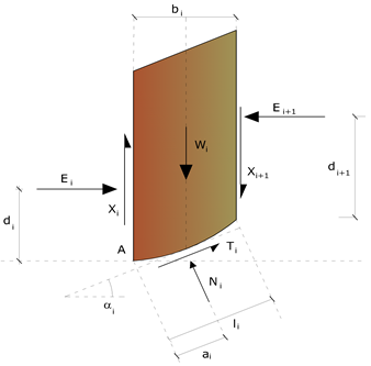
- (n-1) normal forces Ei acting on slice interface;
- (n-1) tangential forces Xi acting on slice interface;
- n values of the coordinate “a” that identifies the point of application of Ei;
- (n-1) values of the coordinate that identifies the point of application of Xi;
- an unknown constituted by the safety factor F.
In all the unknowns are (6n-2). While the equations are:
- equilibrium equations of the moments n;
- equilibrium equations at the vertical displacement n;
- equilibrium equations at the horizontal displacement n;
- equations relative to the failure criterion n.
In all there are 4n equations.
The problem is statistically indeterminate to the extent of:
i=(6n-2)-4n=2n-2
The degree of indetermination is further reduced to (n-2) as it is assumed that Ni is applied at a mid point of the slice, which is equivalent to assume the hypothesis that total normal stresses are distributed uniformly. The various methods that are based on limit equilibrium theory differ in the way in which the (n-2) degrees of indetermination are eliminated.
Fellenius method (1927)
With this method (only valid for circular form slide surfaces) interslice forces are ignored and thereby the unknowns are reduced to:
- n values of normal forces Ni;
- n values of shear forces Ti;
- 1 safety factor.
Unknows (2n+1). The available equations are:
- n equilibrium equations at the vertical displacement;
- n equations relative to the failure criterion;
- 1 equation of the global moments.
F={Σì[ci·li+(Wi·cosαi-ui·li)·tanφi}/(Σì·sinαi)
This equation is easy to solve, but it was found that provides conservative results (low safety factors) especially for deep surfaces or at the increase in the value of the pore pressure.
Bishop method (1955)
None of the contributing forces acting on slices is ignored using this method that was the first to describe the problems of conventional methods. The equations used to resolve the problem are:
Σ Fy=0 Σ M0=0 Failure criterion
 F={Σì[ci·bi+(Wi-ui·bi+ΔXi)·tanφi]·[secαi/(1+tanαi·tanφi/F)]}/(ΣìWi·sinαi)
The values of F and ΔX for each item that satisfy this equation give a rigorous solution to the problem. As a first approximation should be taken ΔX = 0 and iterate for calculating the factor of safety, this procedure is known as the ordinary method of Bishop, the errors made compared to the complete method are about 1%.
Janbu method (1967)
Janbu has extended Bishop’s method to freeform surfaces. When freeform (generic form) sliding surfaces are treated, the arm of the forces changes (in case of circular surfaces it is constant and equal to the radius of the arc) and therefore it is more convenient to evaluate the moment equation at the angle of each slice.
F={Σì[ci·bi+(Wi-ui·bi+ΔXi)·tanφi]·[sec^(2)αi/(1+tanαi·tanφi/F)]}/(ΣìWi·tanαi)


Assuming ΔXi = 0 is obtained by the ordinary method. Janbu also proposed a method for the correction of the safety factor obtained by the ordinary method according to the following:
Fcorretto=f0·F
where f0 empirical correction factor, depends on the shape of the sliding surface and on the geotechnical parameters. This correction is very reliable for slightly inclined slopes.


Bell method (1968)
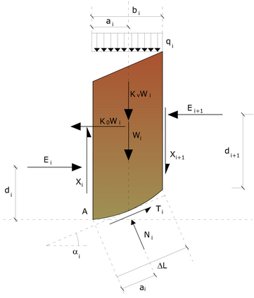
The forces acting on the mass that slides include the weight of soil, W, seismic horizontal and vertical pseudo static forces Kx·W e Ky·W, , the horizontal and vertical forces X and Y applied externally to the slope profile, the resultant of the total normal and shear stresses σ and τ acting on the potential sliding surface.
The total normal stress can include an excess of the pore pressure u that must be specified with the introduction of the parameters of effective force. In practice, this method can be considered as an extension of the method of the circle of friction for homogeneous sections previously described by Taylor. In accordance with Mohr-Coulomb theory in terms of effective stress, the shear stress acting on the base of the i-th slice is given by:
Ti=[ci·Li+(Ni-uci·Li)·tanφi]/F
where:
F = safety factor;
ci = the effective cohesion (or total) at the the base of the i-th slice;
φi = the effective friction angle (= 0 with the total cohesion) at the the base of the i-th slice;
Li = the length of the base of the i-th slice;
uci = the pore pressure at the center of the base of the i-th slice.
The equilibrium is obtained by equating to zero the sum of the horizontal forces, the sum of the vertical forces and the sum of the moments compared to the origin.
It is adopted the following assumption on the variation of the normal stress acting on the potential sliding surface:
σci=[C1·(1-Kz)·(Wi·cosαi)/Li]+C2·f(xci,yci,zci)
Wi·cosαi/Li= total value of the normal stress associated with the ordinary method of the slices
The second term of the equation includes the function:
f=sin2π·[(xn-xci)/(xn-x0)]
Where x0 and xn are respectively the abscissa of the first and the last point of the sliding surface, while xci are respectively the abscissa of the first and the last point of the sliding surface, while. A sensitive part of weight reduction associated with a vertical acceleration of the ground Ky g g can be transmitted directly to the base and this is included in the factor (1 – Ky). The total normal stress at the base of a slice is given by:
Ni= σci ·Li
The solution of the equations of equilibrium is obtained by solving a linear system of three equations obtained by multiplying the equilibrium equations for the safety factor F , substituting the expression of Ni and multiplying each term of the cohesion by an arbitrary factor C3. Any pair of values of the safety factor in the close to a physically reasonable estimate can be used to initiate an iterative solution. The required number of iterations depends on the initial estimate and the desired accuracy of the solution, normally, the process converges rapidly.
Sarma method (1973)
The method of Sarma is a simple, but accurate method for the analysis of slope stability, which allows to determine the horizontal seismic acceleration required so that the mass of soil, delimited by the sliding surface and by the topographic profile, reaches the limit equilibrium state (critical acceleration Kc) and, at the same time, allows to obtain the usual safety factor obtained as for the other most common geotechnical methods.
It is a method based on the principle of limit equilibrium of the slices, therefore, is considered the equilibrium of a potential sliding soil mass divided into n vertical slices of a thickness sufficiently small to be considered eligible the assumption that the normal stress Ni acts in the midpoint of the base of the slice.
The equations to be taken into consideration are:
- The equation of equilibrium to the horizontal translation of the single slice;
- The equation of equilibrium to the vertical translation of the single slice;
- The equation of equilibrium of moments.
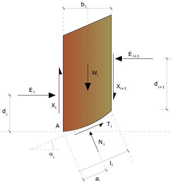
Equilibrium conditions to horizontal and vertical translation:
Ni·cosαi+Ti·sinαi=Wi-ΔXi
Ti·cosαi-Ni·sinαi=KWi-ΔEi
It is also assumed that in the absence of external forces on the free surface of mass occurs:
Σ ΔEi = 0
Σ ΔXì = 0
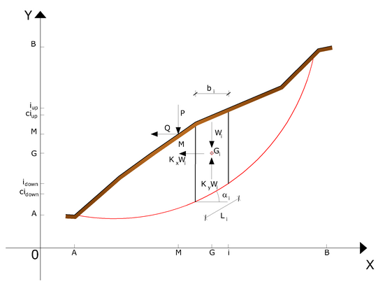
where Ei e Xi represent, respectively, the horizontal and vertical forces on the face of the generic slice i. The equilibrium equation of moments is written choosing as a reference point the center of gravity of the entire mass; so that, after performing a series of trigonometric and algebraic positions and transformations, the solution of the problem in Sarma method passes through the resolution of two equations:
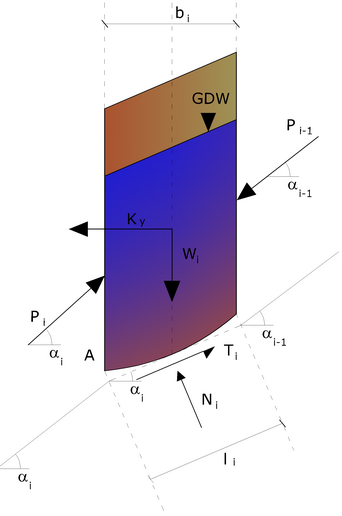
Actions on the i-th slice according to Sarma
Σ ΔXì·tan(ψi– αi)+Σ ΔEi=Σ Δi-KWi
Σ ΔXì·[(ymi-yG)·tan(ψi– αi)+(xmi-xG)]=Σ Wì ·(xmi-xG)+Σ Δi-(ymi-yG)
But the solution approach, in this case, is completely inverted: the problem in fact makes it necessary to find a value of K (seismic acceleration) corresponding to a given safety factor; and in particular, find the acceleration value K corresponding to the safety factor F = 1, that is, the critical acceleration.
Therefore:
K=Kc Critical acceleration if F=1
F=Fs Safety factors in static condition if K=0
The second part of the problem of Sarma’s method is to find a distribution of internal forces Xi and Ei such as to verify the equilibrium of the slice and the global equilibrium of the whole body, without breach of the failure criterion. It has been found that an acceptable solution of the problem can be achieved by assuming the following distribution for the Xi forces:
ΣΔXì=λ·ΔQì=λ·(Qì+1-Q1)
where Qi is a known function, in which are taken into consideration the average geotechnical parameters on the i-th face of the slice i, and l represents an unknown. The complete solution of the problem is obtained therefore, after a few iterations, with the values of Kc, l and F, that allow to obtain even the distribution of interslice forces.
Spencer method (1967)
The method is based on the following assumptions:
- the interslice forces along the division surfaces of the individual slices are oriented parallel to one another and inclined compared to the horizontal by an angle θ;
- all moments are null Mi =0, i=1…..n.
Basically, the method satisfies all the statics equations and is equivalent to the method of Morgenstern and Price when the function f(x) = 1. Imposing the equilibrium of moments from the center of the arc described by the sliding surface:
1) ΣQì·R·cos(α-θ)=0
where:

Qì=0
interaction force between the slices;
R = radius of the arc of the circle;
θ = angle of inclination of the force Qi from the horizontal.
Imposing the equilibrium of horizontal and vertical forces we have respectively:
Σ(Qì·cosθ)=0
Σ(Qì·senθ)=0
With the assumption of Qi forces parallel to each other, we can also write:
2) ΣQì=0
Qì={c/Fs·(W·cosα-γw·h·l·secα)·tanα/Fs-W·sinα}/{cos(α-θ)·[(Fs+tanφ·tan(α-θ)]/Fs}
The method proposes to calculate two safety factors: the first (Fsm) obtainable from 1), related to the equilibrium of moments, the second (Fsf) dalla 2)obtainable from 2) related to the equilibrium of forces. In practice, we proceed by solving 1) and 2) for a given range of values of the angle θ, considering as a unique value of the safety factor that for which:
Fsm=Fsf
Method of Morgenstern e Price (1965)
A relation is established between the components of the interslice forces of the type X = λ f(x)E, where λ is a scale factor and f(x), function of the position of E and X, defining a relation between the variation of the force X and the force E inside the sliding mass. The function f(x) is arbitrarily chosen (constant, sine, half-sine, trapezoidal, etc.) and has little influence on the result, but it should be verified that the values obtained for the unknowns are physically acceptable.
The particularity of the method is that the mass is divided into infinitesimal strips to which are imposed the equations of equilibrium to the horizontal and vertical translation and failure on the basis of the strips themselves. This leads to a first differential equation that binds interslice unknown forces E, X, the factor of safety Fs,the weight of the infinitesimal strip dW and the resultant of the pore pressure at the base dU.
The result is the so-called “equation of forces”:
c’·(α/Fs)+tanφ’·[(dW/dx)-(dX/dx)-tanα(dE/dx)-secα·(dU/dx)]=(dE/dx)-tanα·[(dX/dx)-(dW/dx)]

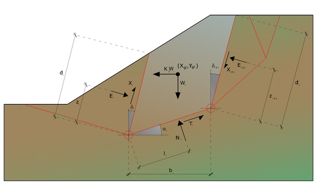
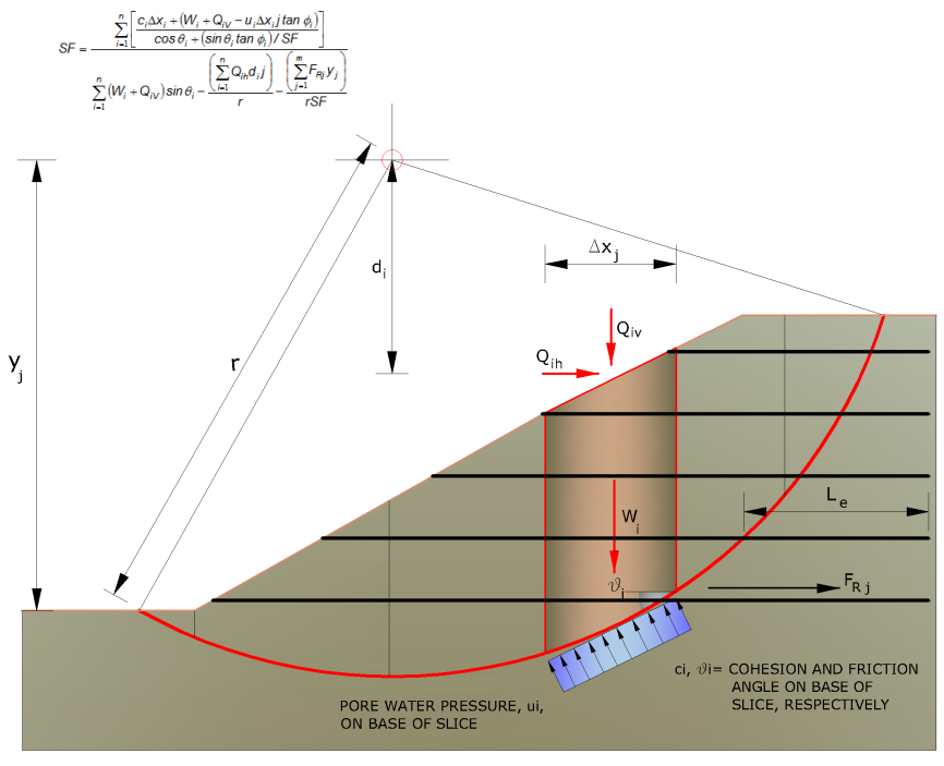
Actions on the i-th slice according to Morgenstern & Price add representation of the entire mass
A second equation, called “equation of moments”, is written by imposing the condition of equilibrium to rotation with respect to the middle of the base:
X=d(Eγ)/dx-γ·dE/dx
these two equations are extended by integration at the whole mass concerned from sliding.
The calculation method satisfies all equilibrium equations and is applicable to surfaces of any shape, but not necessarily imply the use of a computer.
Method of Zeng e Liang (2002)
Zeng and Liang carried out a series of parametric analyzes of a two-dimensional model developed by finite element code, which reproduces the case of drilled shafts (piles immersed in a moving soil). The two-dimensional model reproduces a slice of soil of unit thickness and assumes that the phenomenon occurs in plane strain conditions in the direction parallel to the axis of the piles. The model was used to investigate the influence on the formation of an arch effect of some parameters such as the distance between the piles, the diameter and the shape of the piles, and the mechanical properties of the soil. The authors identify the relation between the distance and the diameter of the piles (s/d), the dimensionless parameter determining the formation of the arch effect. The problem appears to be statically indeterminate, with degree of indeterminacy equal to (8n-4), but in spite of this it is possible to obtain a solution by reducing the number of unknowns and thus taking simplifying assumptions, in order to make determined the problem..
The assumptions that make the problem determined are:
-Ky are taken horizontal to reduce the total number of unknowns with (n-1) to (7n-3);.
-Le normal forces at the base of the strip acting in the midpoint, reducing the unknowns with n to (6n-3);
-The position of the lateral thrusts is to one-third of the average height of inter-slice and reduces the unknowns with (n-1) to (5n-2);
-The forces (Pi-1) and Pi are assumed parallel to the inclination of the base of the strip (αi), reducing the unknowns with (n-1) to (4n-1);
-It is assumed a single yield constant for all the slices, reducing the unknowns with (n) to (3n-1).
The total number of unknowns is then reduced to (3n), to be calculated using the factor of load transfer. Furthermore it should be noted that the stabilization force transmitted on the soil downhill of the piles is reduced by an amount R, called reduction factor, calculated as:
R=[1/(s/d)]+{1-[1/(s/d)]}·Rp
The factor R therefore depends on the ratio between the distance present between the piles and the diameter of the piles and by the factor Rp which takes into account the arch effect.
Evaluation of the seismic action
The slope stability against seismic action is checked with the pseudo-static method. For soils that under the action of a cyclic loading can develop high pore-water pressure is considered an increase in percent of pore-water pressures that takes account of this factor of loss of resistance.
For the assessment of the seismic forces are considered the following:
FH=Kx·W
FV=Ky·W
Where:
- FH and FV respectively the horizontal and vertical component of the inertial force applied to the center of gravity of the slice.
- W slice weight;
- Kx horizontal seismic coefficient;
- Ky vertical seismic coefficient.
Search of the critical sliding surface
In the presence of homogeneous mediums there are no available methods for detecting the critical sliding surface and must examine a large number of potential surfaces.
In case of circular shape surfaces, the search becomes more simple, since after placing a mesh of centers consisting of m rows and n columns will be examined all surfaces having as center the generic node of the mesh m´n and variable radius in a given range of values that examine surfaces kinematically admissible. .
Stabilization of slopes using piles
The realization of a row of piles on a slope serves to make increase the shear strength of certain sliding surfaces. The intervention may be consequent to a stability already ascertained, for which you know the sliding surface or, acting preventively, is designed in relation to hypothetical sliding surfaces which responsibly can be assumed as the most probable ones. In any case is assumed a mass of soil moving on a stable mass on which to attest, for a certain length, the alignment of piles.
The soil, in the two areas, has a different influence on the uniaxial element (pile): stresses at the top (passive pile – active soil) and resistive in the area below ground level (active pile – passive soil). From this interference between “barrier” and moving mass, are developed stabilizing actions that must pursue the following objectives:
- give the slope a safety factor greater than that initial;
- be absorbed by the work, ensuring its integrity (internal tensions, arising from the maximum stresses transmitted over different sections of the single pile, must be less than the allowable tensions of the material) and be below the tolerable limit load of the ground that is calculated considering the interaction (pile-soil).
Limit load related to the interaction between piles and lateral terrain
In the various types of soil that don’t have a homogeneous behavior, the deformations at the contact area are not connected to each other.
Therefore, unable to associate to the material a perfectly elastic pattern behavior (hypotheses that could be taken for slightly fractured stone materials), generally is imposed that the mass movement is in the initial state and that the soil adjacent to the piles is in the maximum allowed phase of yield, beyond which might be encounter the undesirable effect that the material can flow through the row of piles, in the space between an element and another.

Imposing also that the load absorbed by the soil is equal to that associated with the hypothesized limit condition and that between two consecutive piles, as a result of the active thrust, will establish a sort of arch effect, the authors T. Ito and T. Matsui (1975) have derived the relationship that allows to determine the limit load. The limit load is reached by reference to the static scheme, designed in the previous figure and to the assumptions mentioned above, that are reaffirmed schematically.
- Under the action of the active pressure of the earth are formed two sliding surfaces corresponding to lines AEB and A’E’B.
- The dirrections EB and E’B’ form with the axis x the angles +(45 + φ/2) respectively –(45 + φ/2).
- The mass of soil, within the area delimited by the vertices AEBB’E’A’, has a plastic behaviour, so the application of the Mohr-Coulomb failure criterion is allowed.
- The active earth pressure acts on the A-A’ plane.
- The piles have high bending and shear stiffness.
The expression, referring to the generic Z depth, relatively to a unit ground thickness, is:
P(Z)=C·D1·(D1/D2)^(k1)·{1/[(Nφ·tanφ)·(e^(k2)-2(Nφ)^(0.5)·tanφ-1)]}-C·[D1·k3-D2/(Nφ)^(0.5)+γ·Z/{Nφ-[D1·(D1/D2)^(k1)·e^(k2)-D2]}
where the symbols used have the following meaning:
C = soil cohesion;
φ = friction angle;
γ = soil specific weight;
D1 = interaxis between piles;
D2 = sgap between two consecutive poles;
Nφ = tag2(π/4 + φ/2)
K1=Nφ^(0.5)·tanφ+Nφ-1
K2=[(D2-D1)/D2]·Nφ·tan(π/8 + φ/4)
K3=[2·tanφ+2·Nφ^(0.5)+1/Nφ^(0.5)]/[Nφ^(0.5)·tanφ+Nφ-1]
The total force, relatively to a layer of soil in motion of thickness H, was obtained by integrating the above expression.
In the presence of granular soils (drained condition), in which we can assume C = 0, the expression becomes:
P(Z)=[0.5·γ·H^(2)]/{Nφ[D1·(D1/D2)^(k1)·e^(k2)-D2]}
For cohesive soils (undrained conditions), with φ = 0 and C ≠ 0, we have:
P(Z)=C·{D1·[3·ln(D1/D2)+(D1-D2)/(D2)·tanπ/8]-2·(D1-D2)}+γ·z·(D1-D2)
P=ſ0,HP(z)·dz
P(Z)=C·H·{D1·[3·ln(D1/D2)+(D1-D2)/(D2)·tanπ/8]-2·(D1-D2)}0.5·γ·H^(2)·(D1-D2)
The dimensioning of the curtain of piles, which, as already mentioned, must confer an increase of the slope factor of safety and guarantee the integrity of the pile-soil mechanism, is quite problematic. In fact, given the complexity of the expression of the load P, influenced by several factors related both to the mechanical characteristics of the ground and to the geometry of the work, it is not easy with a single processing to reach the optimal solution. To achieve this it is necessary, therefore, to perform several attempts aimed to:
- Find, on the topographic profile of the slope, the location that provides, equally to other conditions, a more comforting distribution of safety factors.
- To determine the planimetric arrangement of the piles, characterized by the ratio between the interaxis and the distance between the piles (D2/D1), that allows to take the most advantage of the resistance of the pile-soil complex; experimentally it was found that, excluding limit cases (D2 = 0, P → ∞ and D2 = D1 P → minimum value), the values are most suitable for the purpose are the ones for which this ratio lies between 0.60 and 0.80.
- To assess the possibility of incorporating more rows of piles and possibly, if so, to determine, for subsequent rows, the position that gives more guarantees in terms of safety and waste of materials.
- To adopt the most suitable type of bond that allows obtaining a more regular distribution of stresses; experimentally it was found that the bond that fulfills, in a more satisfactory manner, the purpose is the bond that prevents the rotations to the head of the pile.
Broms limit load method
In the case in which the pile is loaded orthogonally to the axis, load configuration present if a pile inhibits the movement of a sliding mass, the resistance can be entrusted to its horizontal load limit.
The problem of calculating the horizontal limit load has been addressed by Broms both for the purely cohesive medium that the for incoherent medium. The computation method is based on some simplifying assumptions with regard to the reaction exerted by the ground per unit length of pile in limit conditions and leads into account also the shear strength of the pile (Yield moment).
Reinforcing element
The reinforcements are horizontal elements placed on the ground to confer a greater resistance to sliding.
If the reinforcing element intersects the sliding surface, the resisting force developed by the element in considered in the equilibrium equation of the single slice, otherwise the reinforcing element does not influence the stability..
The internal verifications have the purpose of assessing the stability level of the reinforced mass; the calculated ones are failure verification of the reinforcing element due to tensile stress and pullout verification. The parameter that provides the tensile strength of the reinforcement,TAllow, is calculated from the nominal resistance of the material used to manufacture the reinforcement, reduced by suitable coefficients which take into account the aggressiveness of the soil, damage due to creep and damage due to installation.
The other parameter is the pullout resistance that is calculated through the following relation:
TPullout=2·Le·σ’v·fb·tanδ
For closed mesh geotextile
fb=tanδ/tanφ
where:
δ Represents the angle of friction between soil and reinforcement element.
TPullout Resistance mobilized by a reinforcement anchored by a length Le within the stable part of the soil.
Le Anchorage length of the reinforcement within the stable part.
fb Pullout coefficient.
σ’v Vertical stress, calculated at the average depth of the reinforcement section anchored to the ground.
Is chosen the minimum value between TAllow and TPullout, the internal verification will be satisfied if the force exerted by the reinforcement, generated on the back of the reinforced section, does not exceed the value of T ‘.
Anchors
The anchors, bolts or nails, are the structural elements capable of withstanding tensile forces by virtue of an appropriate connection to the ground.
The characteristic features of an anchor are:
- head: indicates the set of elements that have the function of transmitting to the anchored structure he tensile stress of the anchor;
- foundation: indicates the part of the anchor that makes the connection with the ground, transmitting the ground tensile stress of the anchor.

Completly anchored bulb
Partially anchored bulb
The section between the head and the foundation is called the free part, while the foundation (or bulb ) is made by injecting the mortar, generally cement, into the soil. The soul of the anchor consists of an armature, made of rods, wires or strands.
The anchor intervenes in the stability in a greater or lesser effectiveness depending whether it will be totally or partially (the case where it is intercepted by the sliding surface) anchored to the stable part of the soil.
The relationships which express the security measure along a hypothetical sliding surface will change in the presence of anchors (active anchor, passive anchor and nails) in the following way:
- for active anchors, their resistance will be deducted from the shares (denominator)
FS=Rd/[Ed-Σi,jRi,j·(1/cosαi)]
- for passive anchors and nails, their contribution is summed to the resistances (nukerator)
FS=[Rd+Σi,jRi,j·(1/cosαi)]/Ed
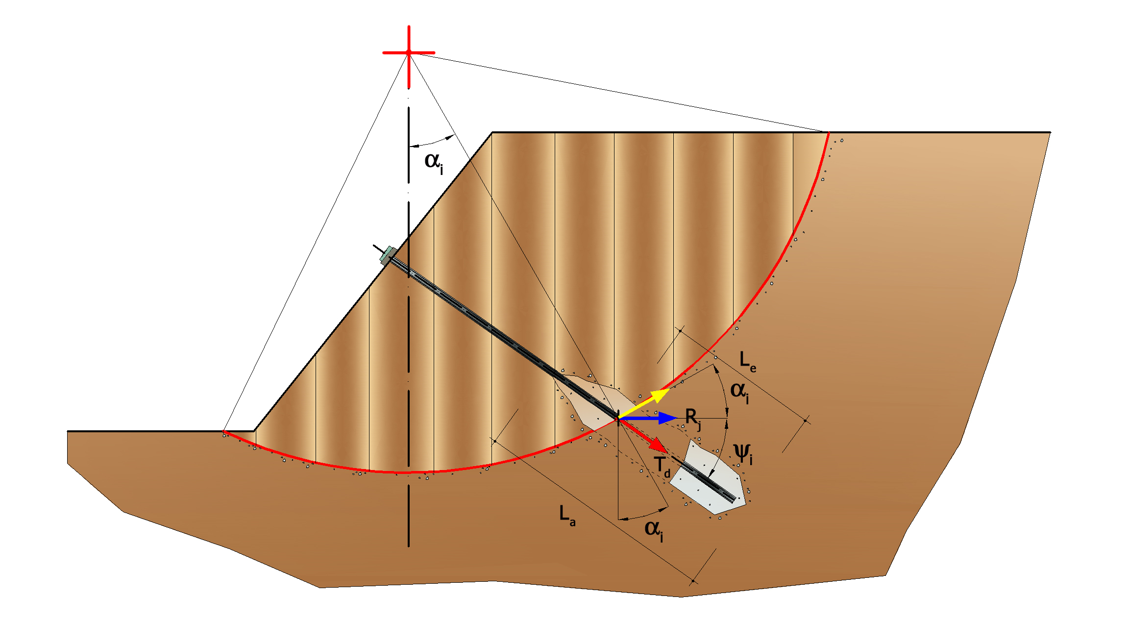
- Rj indicates the anchor strength and it is calculated using the following expression:
Rj=Td·cosΨi·(1/i)·(Le/La)
Where:
Td design strength
Ψ i anchor inclination relative to the horizontal
i interaxis
Le effective length
La anchored (bulb) length
The two indexes (i, j) in the sum represent the ith slice and the jth anchor intercepted by the sliding surface of the ith slice.
Extract of the technical report of SLOPE